Example 5.11 models one‑dimensional transient heat conduction in a fuel element of a nuclear reactor that is in the shape of a plane wall with a thickness 2L = 20 mm and is convectively cooled on both surfaces. A space increment of Δx = 2 mm is used, so that the half‑thickness is discretized into a finite‑difference nodal network with 6 unknown nodal temperatures. Each node represents a control volume of the fuel element, and the temperatures at these nodes are obtained using the energy balance method.
The wall generates heat uniformly at a specified volumetric rate, and both surfaces are exposed to the same convection conditions, characterized by a convection coefficient h and ambient temperature T∞. For each interior node, an unsteady energy balance is written that includes transient energy storage, conduction to adjacent nodes, and uniform internal heat generation. At the two surface nodes, the energy balance also includes convective heat loss terms. These node‑type equations follow the explicit finite‑difference form for 1‑D transient conduction with convection boundaries and are implemented in MATLAB as a time‑marching scheme to determine how the temperature distribution evolves after a sudden change in heat generation.
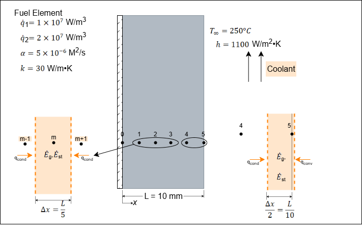
Figure 5 – Nodal network for Example 5.11